An end-to-end project for California's Housing Prices

Now we will tackle our first machine learning project, which would involve predicting housing prices in California based on data from 1990s.

The author lists a bunch of data repositories and a checklist for anyone working on a machine learning project, but I will list all of that in some other note.

Roughly, the steps here are:

1. Look at the big picture.
2. Get the data.
3. Explore and visualize the data to gain insights.
4. Prepare the data for machine learning algorithms.
5. Select a model and train it.
6. Fine-tune your model.
7. Present your solution.
8. Launch, monitor, and maintain your system.

Task: build a model for housing prices for the state

Framing the problem

It turns out in this hypothetical scenario that the model we will be developing will be a part of a larger pipeline, where housing prices from our model and other signals¹ will be fed into another ML system which would decide whether it’s worth investing in a given area. The author wants to illustrate the idea that you should have a rough idea of how your model fits into the big picture. There’s also a neat a project checklist in the appendix, but more on that later.

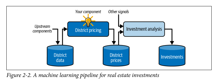
Pipelines

A sequence of data processing components, usually self-contained, is called a data pipeline. Every component pulls in some data, and spits out an output.

Settling on a model type: This should be a classic supervised task as the training data (from 1990s) should contain labels for what the housing prices were for a given population. The model needs to predict this outcome for new populations, and that should be a task for a particular type of supervised learning - regression. Online or batch is something I don’t think has been made obvious by the problem statement. If we want to predict for new data on the fly, online is preferred, but here batch should be the way to go as we have to do some investment analysis on it, and populations won’t change (by a sizable margin) over a relatively long period of time (time b/w consensus).

Author’s answer: supervised, regression - multiple regression as we’re utilising multiple features, and univariate regression as we will emit one output (the price), otherwise it would’ve been multivariate. And they chose to go for plain batch learning. They also suggest that if the data were huge you could use online learning or distribute the computation across multiple systems using something like MapReduce.

Selection of a performance measure: It seems that RMSE (root mean squared error) is the go to performance measure for regression problems.

Some

• m is the number of instances in the dataset you’re measuring RMSE on. Ex. on a validation set of 2000 districts, m = 2000.
• is the vector of all feature values of the ith instance while is the desired label. Ex. f the first district in the dataset is located at longitude –118.29°, - latitude 33.91°, and it has 1,416 inhabitants with a median income of 38,372, and the median house value is 156,400 (ignoring other features for now), then:
  
  and
  
• thus, this keeps the dataset “shape” in mind (elaborate)
• is the matrix containing all feature values excluding labels for all instances of the dataset. There is one row per instance and the ith row is equal to the transpose (flipping rows and columns) of .
  
• h is a hypothesis or this system’s prediction function. When given an instance’s feature vector it emits an output
  Prediction error here is given as: .
• is then the cost function measured on this set of examples using hypothesis h.

In the case of many outliers Mean Absolute Error (MAE) is preferred instead:

Distance measures are also called norms, and they’re of many kinds, ex. l1 norm and l2 norm. More information in Norms and Spaces.
The norm of a vector is defined as:

gives number of non-zero elements and gives max. absolute value in the vector.

TIP

The higher the norm index the more it focuses on large values and negelects small ones.
RMSE uses the norm or Euclidean norm while MAE uses the norm.
Thus in case of more outliers RMSE is likely to miss some values because of its focus on larger values. Then MAE is used. But generally when data is distributed normally RMSE performs really well.

Lastly, check the assumptions and verify what you’re going to be working with and the nature of output you’d be feeding downstream before you actually start working.

Some definitions

Stratified sampling: data is divided into homogeneous subgroups called strata and the right number of instances are sampled from each stratum to guarantee that the test set if representative of the data as a whole. Ex. when people conduct a survey of 1000 people, they don’t just pick those people randomly but try to make sure that these 1000 people are representative of the whole population, ex. if the US population is 51.1% females we would try to maintain a ratio of 511 females and 489 males.
In this project we use Scikit-Learn’s builtin train_test_split function with the parameter stratify set to some attribute in our data frame.

Correlation coefficient: aka Pearson’s . It measures linear correlation (“as x goes up y generally goes up/down”) and ranges from -1 to 1. When it’s close to 1 it means that there is a strong positive correlation, ex. in our dataset the median house value tends to go up when median income goes up. When it’s close to -1 there is a strong negative correlation, ex. if x goes up y goes down, or inverse proportionality. When it’s close to 0 it means that there is no linear correlation. TRAP: It may completely miss out on nonlinear relationships, ex. “as x approaches 0 y generally goes up.”
We use the pd.DataFrame.corr(numeric_only=True) method to measure the correlation in a pandas data frame.

Imputation: Part of data cleaning where we substitute a missing value with some other value, ex. zero, mean, median, etc. In a simple implementation we can use pandas Data Frame’s fillna() method, but the Scikit Learn class SimpleImputer is better for this use case, as it stores the median value of each feature in a special variable statistics_ and can be used to substitute the median in place of the empty values when we actually “transform” the data frame. Missing values can also be substituted by the mean or the most frequent value or a constant value. See the documentation for more details.

Categorical attributes: attributes that can acquire a limited number of possible values, each of which represent a category (ex. “good”, “bad”, “average”, etc.). We use encoding to handle categorical attributes. But if a categorical attribute has a large number of possible categories (ex. country code, profession, species) then one-hot encoding will result in a large number of input features. If this happens, we may replace the categorical attribute with numerical features related to the categories (ex. ocean_proximity with distance from ocean, country code with country’s population and GDP per capita). When dealing with neural networks, we can replace each category with a learnable, low-dimensional vector called an embedding.

Encoding: Conversion of categorical attributes to numbers so that machine learning algorithms are able to work with that data. See the documentation for each.

• Ordinal encoding: We use the OrdinalEncoder class for this. Here, we encode categorical features as an integer array. There is however a problem with this; machine learning algorithms can assume that two “nearby” values are more similar than two distant values. This is fine in some cases, ex. for ordered categories, “bad”, “average”, “good” and “excellent” but it’s not the case in our project here, where in the ocean_proximity column the categories <1H OCEAN and OCEAN were similar but were still assigned 0 and 4 respectively during ordinal encoding. To resolve this, we use one-hot encoding.

• One-hot encoding: A technique used to convert categorical data into a binary format where each category is represented by a separate column with a 1 indicating its presence and 0s for all other categories. This is called one hot encoding because only one attribute will be equal to 1 (hot), while others will be 0 (cold). The new attributes are called dummy attributes. 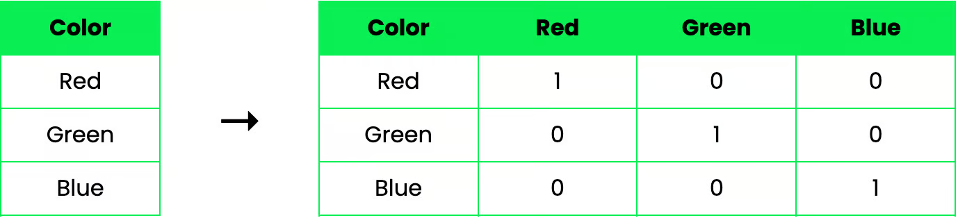We use the OneHotEncoder class to implement this. Indeed, this results in a sparse matrix where most of the elements are zero; it’s an efficient representation of a matrix that contains mostly zeros. To convert the sparse matrix to a (dense) numpy array we use the toarray() method. We can also set the sparse_output hyperparam to False in order to get a regular numpy array directly. The advantage of using OneHotEncoder over pandas.get_dummies() is that it “remembers” each categorical attribute. See HOML pg 73 for an example.

• Feature scaling: scaling features so that all of them have approximately the same scale.

  • Min-max scaling: aka normalization. For each attribute, the values are shifted and rescaled so that they end up ranging from 0 to 1. This is performed by subtracting the min value and dividing by the difference between the min and the max value. We use the transformer MinMaxScaler for this.
  • Standardization: It subtracts the mean value (so standardized values have a zero mean) and then it divides the result by the standard deviation (so standardized values have SD = 1). It does not restrict values to a specific range, like min-max scaling. It is much less affected by outliers. We use the transformer StandardScaler for this.
  • Heavy tail shrinking: when a feature’s distribution has a heavy tail, or when values far from the mean are not exponentially rare, both min max scaling and standardization will squash most values into a small range. So before scaling the feature, we first transform it to shrink the heavy tail and if possible make the distribution roughly symmetrical (ex. Gaussian). For ex. replacing the feature with its square root (or any power b/w 0 and 1). If a feature has a really long and heavy tail, such as in power law distributions, we replace it with its logarithm.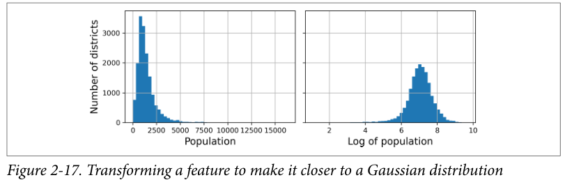Another approach towards handling heavy-tailed features is bucketization or chopping the distribution into equally sized blocks and replacing each feature value with the id of the bucket it belongs to. This results in an almost uniform distribution. When a feature has a multimodal distribution (a bunch of peaks), we can bucketize that too but this time we could treat bucket IDs as categories and not just numerical values. We could even encode the bucket indices using a onehot encoder for example. This would allow the model to learn different rules for different ranges for this feature value.
  • Radial basis function: any function that depends only on the distance between the input value and a fixed point. The most commonly used RBF is the Gaussian RBF whose output value decays exponentially as the input moves away from the fixed point. For ex. gives the Gaussian RBF similarity between housing age x and 35.

• Inverse transformers : Used to compute the inverse of a transformation. We do this when we transform the target values; if the target distribution has a heavy tail, we may replace it with its log, and accept the fact that the model will low predict the log of the target value, not the value itself, and inverse transform the model’s outputs to get the real target value.

• Root mean squared error: Why is it squared? That’s something to think about. We have discussed RMSE before, so see that discussion for the formula. Here we use the root_mean_squared_error method from sklearn.metrics to measure the RMSE. In the docs this function returns a “loss” which is defined as a non negative floating point value whose best value is 0.0.

• k-fold cross validation: the training set is divided into k subsets called folds (all containing different data and thus non overlapping), and then it would train and evaluate the model k times, each time selecting one of the k subsets as a validation set. It would then provide you with an array of k validation scores. We use the cross_val_score method for it. NOTE: the cross validation feature expects a utility function (greater is better) rather than a cost function (lower is better). RMSE was a cost function so we will need to switch the sign of the cross_val_score in order to get the RMSE score in this particular example. See cell 78 in my notebook.

• Randomized search: This is used when hyperparameter search space is large. Grid search restricts us to only those combinations of params that we have provided ourselves, while in randomized search instead of trying out all possible combinations it evaluates a fixed number of combinations, selecting a random value for each hyperparameter at every iteration. This has several benefits, such as if some of our hyperarams are continuous and we let randomized search run for 1000 iterations, it will explore 1000 different values while grid search would only explore the few values I listed for each one. Also, if there are 6 hyperparameters to explore, each with 10 possible values, then grid search offers no other choice than training a model one million times, whereas random search can always run for any number of iterations we choose. In randomized search, for each parameter, we provide either a list of possible values or a probability distribution.

• Halving search: HalvingRandomSearchCV and HalvingGridSearchCV’s goal is to use the computational resources more efficiently, either to train faster or explore a larger hyperparam space. In the first round they take many hyperparam combinations, called candidates using either the random or the grid approach. These candidates are then used to train models that are evaluated by cross validation. Once we evaluate every candidate, only the best ones proceed to the second round. After several rounds, the final candidates are evaluated using full resources.

• Model rot: If a model was trained on last year’s data, it may not be adapted to today’s data.

• MLOps: ML Operations - dealing with all the infrastructure involved in machine learning - deploying and maintaining machine learning models efficiently.

Rationale behind some decisions

• Test set: The human brain is great at pattern recognition. And for reasons described in The machine learning landscape, we create a test set to “hide” data from both us and the algorithms in order to save it for later to actually test the model on unseen data.
• Data visualisation or exploration: We do this get an in-depth understanding of the data we are trying to manipulate.
  • Looking for correlations: We compute the correlation coefficient to find (linear) similarities between the different attributes present in our data. See the correlation coefficient definition for more details.
  • Experimenting with attribute combinations: Some attributes by themselves are not very useful, for example the total number of rooms in a district is not useful by its own; but when we take a ratio of it with the total number of households in the district, we get the total number of rooms per house which is arguably a more useful attribute. We look for correlations again after getting these “new” attributes! This round of exploration does not have to be absolutely thorough, the point is to start off on the right foot and quickly gain insights for a reasonably good first prototype. This is an iterative process though and you may find yourself returning to this exploration step after you have a prototype up and running, in order to gain some new insights.
• Preparing data for machine learning algorithms: We write functions to prepare our data for machine learning algorithms, and this requires various steps. We do this in order to give our algorithms the best version of the data, so that the predictions are closer to the expected values. Generally, the first step is to separate the labels from the other features/predictors, so that we have a clean new predictors data frame to work on. We will be applying many transformations to this new data frame consisting only of predictors.
  • Cleaning the data: Most machine learning algorithms cannot work with missing features, so we take care of just that here. If an attribute has missing values, we have the options to either get rid of the corresponding data values of the attribute, or get rid of the whole attribute, or set the missing values to some other value. The last point is called imputation (see definition).
  • Handling text and categorical attributes: Most machine learning algorithms prefer to work with numbers, so we will have to convert those text attributes, or categories of text attributes to numbers. We can use encoding for this, see the definition.
  • Feature scaling and transformation: Machine learning algorithms generally don’t perform well when input numerical attributes have very different scales. Never use fit() or fit_tranform() for anything else than the training set. Once you have a trained scaler, you can then use it transform() any other set, including the validation set, the test set and new data. While the training set values will always be scaled to the specified range, if new data contains outliers, these may be scaled outside the range. To avoid this set the clip hyperparam to true. We use minmax scaling and standardization to get all attributes to have the same scale.
  • Transformation pipelines: There are many data transformation steps that need to be executed in the right order. We use the Pipeline class to help with such sequences of transformations.
• Actually training the model: We consider many different models for training and see if they are underfitting or overfitting the data. We can also make use of cross validation and have some performance measure like RMSE to see how well certain models are performing.
  • Fine tuning a model: Fine tuning means fiddling with the hyperparameters, and regularizing (constraining) the model to avoid overfitting. We can use some inbuilt Scikit-learn classes to search the best hyperparameter combinations for us. An example of such a class includes GridSearchCV or RandomizedSearchCV, or their halving search counterparts. We could also take the feature importances and drop features that are not that important for the model.
  • Evaluating system on the test set: Here we use the test set as the unknown data set and evaluate our system on it. We can also compute a confidence interval using scipy.bootstrap which computes a two-sided bootstrap confidence interval of a statistic. If we have done a lot of hyperparam tuning, the performance will usually be slightly worse than what was measured during cross validation, because the system becomes fine tuned to perform well on the validation data and will likely not perform well on unknown datasets. If that happens, one must not tweak hyperparameters more.
• Deploying the model: If we want to launch a model we will first polish the code, write documentation, tests. etc. and then deploy it. The most basic way to do this is to save the best model we have trained and transfer the file to our production environment and load it. To save the model, we can use joblib. It’s a good idea to save every model we experiment with so that we can come back easily to any model we want. Once our model is transferred to production, we can load and use it. For this, we first must import the custom classes and functions the model relies on (i.e. transferring the code to production), then load the model using joblib and use it to make predictions. If we want to use this model in production in a website, we want to load the model on server startup. We can also use cloud services like Vertex AI.
  • Monitoring the model: We can write monitoring code to check our system’s live performance at regular intervals. A model can also decay because of model rot. In some cases we can monitor the model ‘s performance from downstream data, for ex. if it’s a part of a recommender system and the number of recommended products drops, the model is likely the culprit. We can also take the aid of human analysis in cases like image classification, where we can get a human to rate them. With LLMs being as good as they are right now, I wonder if taking a “better” model and substituting it for human review is what all the big companies are doing, because delegating to humans is time consuming and expensive.
  • Training on new data: If the data keeps evolving, we will need to update our datasets and retrain the model regularly; automating the process as much as possible certainly helps. Things to automate include collecting fresh data regularly, scripts to train the model and fine tune the hyperparams, evaluating the model compared to the previous model on the updated test set, etc.
  • Keeping backups of models: Make sure to have backups of every model you create and have the process and tools in place to roll back to a previous model quickly in case the new model starts failing. Keeping backups of datasets is also a neat thing, as it allows us to evaluate any model against the previous dataset.

An overview of Scikit-Learn’s design

Review the documentation for any class, instance variable, or method.
See https://scikit-learn.org/stable/glossary.html

We can observe the following design principles in Scikit-Learn’s API:

1. Consistency: All objects share a consistent and simple interface.
   • Estimators: Any object that can estimate some parameters based on a dataset is called an estimator (ex. SimpleImputer). The estimation is performed by the fit() method and it takes a dataset as a parameter, or two for supervised learning (the second one contains the labels). Any other parameter needed to guide the estimation is called a hyperparameter and it must be set as an instance variable, generally via a constructor param. (Ex. SimpleImputer’s strategy hyperparam.)
   • Transformers: Some estimators (such as SimpleImputer) can also transform a dataset and are called transformers. The transformation is performed by the transform() method with the dataset to transform as a param. It returns the transformed dataset. The transformation generally relies on learned parameters, like in SimpleImputer. All transformers also have a method called fit_transform() which is equivalent to calling fit() and then transform(); but sometimes fit_transform() is more optimized and runs much faster.
   • Predictors: Some estimators, given a dataset, are able to make predictions. Ex. LinearRegression model. These have a predict() method that takes a dataset of new instances and returns a dataset of corresponding predictions. It also has a score() method that measures the quality of predictions, given a test set (and the corresponding labels in supervised learning). Some predictors can also measure the confidence of their own predictions.
2. Inspection: All the estimator’s hyperparams are accessible directly via public instance variables (ex. imputer.strategy) and all the estimator’s learned parameters are accessible via public instance variables with an underscore suffix (ex. imputer.statistics_).
3. Nonproliferation of classes: Datasets are represented as NumPy arrays or SciPy sparse matrices, instead of homemade classes. Hyperparameters are just regular python strings or numbers.
4. Composition: Existing building blocks are reused as much as possible. Ex. it’s easy to create a Pipeline estimator from an arbitrary sequence of transformers followed by a final estimator.
5. Sensible defaults: Reasonable defaults are provided for most parameters.

Whenever we say “dataset” in this chapter, we generally mean a pandas Data Frame.

Scikit-Learn transformers output numpy arrays or sometimes SciPy sparse matrices, even when they are fed pandas DataFrames as input. To “fix” this, run sklearn.set_config(transform_output="pandas"), and all transformers will output pandas DF’s when they are fed a DF.

sklearn.set_config(display="diagram") is useful for rendering estimators as interactive diagrams in notebooks.

When we fit any estimator using a DataFrame, the estimator stores the column names in the feature_names_in_ attribute. Then it’s ensured that any DF fed to this estimator after that has the same column names. Transformers also provide get_feature_names_out() as a method that can be used to build a dataframe around the transformer’s output.
ex.

df_output = pd.DataFrame(cat_encoder.transform(df_test),
			columns=cat_encoder.get_feature_names_out(),
			index=df_test.index)

Custom Transformers and Classes in Scikit-Learn

For custom transformers, we use FunctionTransformer , ex.

from sklearn.preprocessing import FunctionTransformer
log_transformer = FunctionTransformer(np.log, np.exp)
log_pop = log_transformer.transform(housing["population"])

If we want our transformer to be trainable (ex. have a fit and transform method) we need to create a custom class (incomplete solution below):

from sklearn.base import BaseEstimator, TransformerMixin
from sklearn.utils.validation import check_array, check_is_fitted
 
class CustomStandardScaler(BaseEstimator, TransformerMixin):
  def __init__(self, with_mean=True):
    self.with_mean = with_mean
 
  def fit(self, X, y=None):
    X = check_array(X) # check if X is an array with finite float values
    self.mean_ = X.mean(axis=0)
    self.scale_ = X.std(axis=0)
    self.n_features_in_ = X.shape[1]
    return self
 
  def transform(self, X):
    check_is_fitted(X) # learned attributes with trailing _
    X = check_array(X)
    assert self.n_features_in_ == X.shape[1]
    if self.with_mean:
      X = X - self.mean_
    return X / self.scale_

1. sklearn.utils.validation gives you functions for input validation
2. pipelines require the fit() method to have two arguments, X and y which is why we need y=None.
3. All estimators set n_features_in in the fit() method and they ensure that the data passed to transform() or predict() has this number of features.
4. fit() always returns self
5. All estimators must set feature_names_in_ in the fit() method when they are passed a Data Frame. All transformers should provide a get_feature_names_out() method as well as an inverse_transform() method when their transformation can be reversed.
6. A custom transformer often uses other estimators in its implementation.

Transformation Pipelines

We use the Pipeline class to create a pipeline for a sequence of transformations.
ex.

from sklearn.pipeline import pipeline
 
num_pipeline = Pipeline([
("impute", SimpleImputer(strategy="median")),
("standardize", StandardScaler())
])
# or, this one doesn't let you name them.
num_pipeline = make_pipeline(SimpleImputer(strategy="median"), StandardScaler())

• When you call the fit() method on a pipeline, it sequentially calls fit_tranform() on all transformers, passing the output of each call as a param in the next call. For the final estimator it just calls the fit method.
• A pipeline exposes the same methods as an estimator.
• Instead of using separate pipelines for numerical columns and categorical columns (ex. one hot encoding), we can use a ColumnTransformer that is capable of handling all columns. We can either list all the attributes or use a make_column_selector class. See the 61st cell in my notebook for more details.

Footnotes

1. A signal is a piece of information being fed to a machine learning system, an idea from by Claude Shannon’s information theory. His theory was that you want a high signal-to-noise ratio. ↩