Continued from Norms and Spaces.
Orthogonal Vectors
In an inner product space , two vectors and are said to be orthogonal if
For ex. vectors are orthogonal in with the inner product taken as the usual dot product of vectors (we have explicitly defined the inner product to be the dot product here).
Orthogonal complement
Let be an inner product space, and , then the orthogonal complement of W, denoted by is the set of vectors in V that are orthogonal to every element in W.
For all vectors :
Ex. in with the inner product taken as the usual dot product of vectors in , if we take , then the orthogonal complement of W is .
- There is no requirement on to be a subspace of . However, is always a subspace of . (WHY?)
- If is also a subspace of , then . This means that every vector can be uniquely written as where .
Orthonormal vectors: Two vectors are orthonormal if they are orthogonal and their norms are equal to 1, i.e. the vectors are unit vectors.
Orthogonal matrix
A square matrix is an orthogonal matrix if and only if its columns are orthonormal so that , which implies that . So the inverse is obtained simply by taking the transpose of the matrix.
Transformations with orthogonal matrices are special because the length of a vector is not changed when transforming it using an orthogonal matrix .
For the dot product, we obtain:
Moreover, the angle between two vectors measure via their inner product (see Norms and Spaces for the formula) is also unchanged when transforming (replacing x with Ax for ex.) both of them using an orthogonal matrix.
This means that these matrices define transformations that are rotations.
Orthogonal basis
In an n-dimensional space, we need n basis vectors, i.e. n vectors that are linearly independent. Consider now an n-dimensional vector space and a basis of . If
we call it an orthogonal basis. Additionally, if we call it an orthonormal basis. In an orthonormal basis, every basis vector has a length/norm = 1.
Orthogonal projection
Let be an inner product space and be a subspace of . Also, let be an orthogonal basis of . (This means that all the vectors in the basis are orthogonal to each other.) Now, the linear mapping
is called the orthogonal projection onto .
Think
What does this formula even mean? Let’s see. Whenever we want to imagine many vectors, it’s better to imagine them as points in a space. I know that the inner product is a generalisation of the dot product. For simplicity’s sake let me treat it as the dot product right now. I also know that the ‘s are just basis vectors in a space . Those ‘s are being summed here. Whenever I take a “linear combination” of basis vectors, the space that the resultant vector lives in is the area “spanned” by the basis vectors, or the span of those vectors. And the numerator in each individual expression is a scalar (because of dot product), the denominator is a scalar too. That means the fractional part is a scalar. What does a scalar being multiplied with a vector do? It literally scales the vector along the direction of itself. This means that we are taking a linear combination of scaled basis vectors to generate another vector. Where does this new vector live? It lives in the area spanned by those basis vectors, which is the subspace itself. Now imagine the vector as a point in space and the subspace as a floor below it. Drop a straight line from to its projection . This is the shortest distance from that vector to the space (proof below). The distance between the vector and any general vector is the norm of . Now go read the fifth property below and see what it’s trying to say, It says that the distance between the vector and its projection is always lesser than or equal to the distance between the vector and any random vector in that same subspace.
ex. (plug and chug): Let and . . Take a vector and define the inner product to be the usual dot product. Then which is equal to .
Some properties; for all :
- or
- (see below)
ex. Find the closest point to in .
Let . We choose the inner product to be the dot product here.
(I used a pen and paper for this.) is the closest point to the given vector in .
Proof: The closest point to the vector is .
- How do we determine if it’s the closest point? Let’s imagine this. If is a vector and is its projection in a vector space , it is the closest point to that vector if the line joining them is exactly 90 degrees, or the line and the plane are orthogonal. If we imagine the vector as floating above the floor , and dropping a straight line at 90 degrees on the floor, the point where it hits the floor is the projection vector.
- Now that we know that the line should be 90 degrees, what even is the line. Let’s take a vector as the vector . This “error vector” is the vector of that points from the floor up to the vector floating in the air. Now this error vector’s dot product with the vectors that form the plane below it should be 0 (for it to be orthogonal). What vectors form the plane below? The plane below is just a span of all the different basis vectors. So I can take where the is any basis vector. Recall that this is an orthogonal basis, so for example is zero.
- Let’s expand the second expression a little bit. . This is because of it being an orthogonal basis and the dot product of with ‘s other than itself being zero. This holds true for any basis vector .
- So on the left expression we get and on the right expression we get the same because of all the different ‘s we multiply with. Hence, their difference is 0.
- Because the dot product is zero, the two (sets of) vectors are orthogonal and hence the distance is the shortest.
Think
Take a vector floating in space. Take its projection and drop a line from the vector to its projection. Now take an arbitrary vector along the plane (floor) of the projection (the subspace ) and call that vector . Now connect the projection with this vector, and the floating point with this vector. Now you have a right angled (just proved) triangle. Take the distance from the vector to the projection to be , the distance from the projection to be and the distance between the vectors and to be . (Note that are norms here but I am omitting the because I don’t want to be that verbose here.) Now consider the Pythagorean theorem:
The distance between the projection and the arbitrary vector was and norm squared can be . So the distance or , which is exactly what property 5 says above.
General projection
A linear mapping that satisfies is called a projection. Such linear mappings are expressed by transformation matrices, the projection matrices where .
Projection onto one-dimensional subspaces (lines)
If we are given a line (1D subspace) through the origin with a basis vector , the line is a one dimensional subspace spanned by . When we project onto , we seek the vector that is closest to . This figure is useful for visualizing such projections.
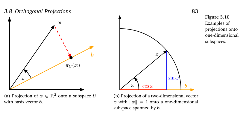
Using geometric arguments,
- the projection is closest to when the distance is minimal. The segment from to is orthogonal to and therefore the basis vector of . The orthogonality condition yields since angles between vectors are defined via the inner product.
- the projection must be an element of and therefore a multiple of the basis vector; hence .
Step A: Finding the coordinate
Since we can have and then we can use the billinearity of the inner product to have . (If you are confused about billinearity just choose the inner product to be the dot product and solve the first equation with the dot product.) Thus we have
Step B: Finding the projection point
Since we can have where the last equality holds true if the inner product is chosen to be the dot product. If we choose the inner product to be the dot product, the following relation holds: , where is the angle between the vectors and . An illustration is shown in (b) of above figure.
Step C: Finding the projection matrix
since if we set the inner product to be the dot product. We see that:
Projections onto general subspaces
Here we will look at projections of vectors onto lower dimensional subspaces with . The illustration for this projection is given below.
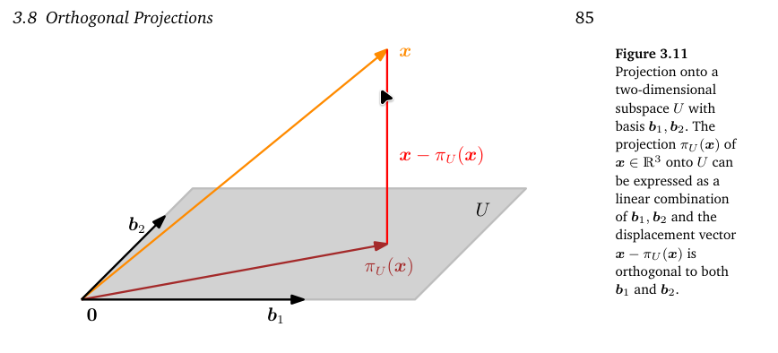
Assume that is an ordered basis of . Any projection onto is necessarily an element of . Therefore, it can be represented as a linear combination of the basis vectors such that .
We can follow a three step procedure again to find the projection and the projection matrix. Note that is a matrix whose columns are the vectors . And also remember that the vector represents the coordinate.
- Find the coordinates of the projection (with respect to the basis of ) such that the linear combination (where are matrices and , ) is closest to . Closest means minimum distance again, which implies that the vector connecting the projection to the original vector, is orthogonal to all basis vectors of . We can thus say that for which we get n simultaneous conditions. Now let’s choose the inner product to be the dot product, and we obtain following the dot product. Using the aforementioned equation, we can write . And since this is of the form This allows us to solve for the coefficients or coordinates, .
- Find the projection. We have already established that . Thus, .
- Find the projection matrix. .
Projections allow us to look at situations where we have a linear system without a solution. This means that does not lie in the span of , i.e. the vector does not lie in the subspace spanned by the columns of . In these cases we need an approximate solution. The idea is to find the vector in the subspace spanned by columns of that is closest to , i.e. we compute the orthogonal projection of onto the subspace spanned by columns of . The solution here is called the least-squares solution of an overdetermined system, as we assume the dot product to be the inner product.
A teaser for machine learning
In that floor analogy above, think of the subspace now, or the floor, as the space of all possible predictions of a machine learning model. Think of the vector as the “true” feature vector we want to have a prediction of. In some models, we use this and we want to find out the most accurate prediction. The most accurate prediction geometrically is the closest point on that floor or plane to the feature vector. This is also the reason we briefly called as the “error” vector, because it represents how off the model is from the prediction.